Tuning
Bias and Variance
1. Define bias within the context of machine learning.
2. Define underfitting within the context of machine learning and the consequence.
Underfitting occurs when the model has high bias, and the model performs poorly on both the training data and new, unseen data.
It fails to capture the complexity of the data, resulting in poor predictive accuracy.
3. Define variance within the context of machine learning.
4. Define overfitting within the context of machine learning and the consequence.
Overfitting occurs when a model has high variance, becomes overly complex, and starts to capture noise or random fluctuations in the training data.
As a result, it fits the training data extremely well but performs poorly on new, unseen data because it has essentially memorised the training data instead of learning generalisable patterns.
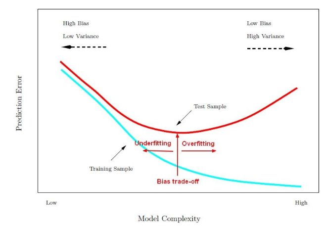
5. Provide a visual diagram to show the bias trade off using training and test curve, where the X-axis = Model Complexity and Y-axis = Prediction Error.
6. On a learning curve chart with epochs on X-axis and error on Y-axis, describe underfitting signs.
- High training error
- High validation error
- Flat learning curve
- No convergence
7. On a learning curve chart with epochs on X-axis and error on Y-axis, describe overfitting signs.
- Decreasing training error
- Increasing validation error
- Noisy learning curve
- Large gap between training and validation error
8. On a learning curve chart with epochs on X-axis and error on Y-axis, describe the signs of a good fitting model.
- Decreasing training error
- Decreasing validation error
- Stable learning curve
- Convergence in training and validation error.
9. What does it mean to find the appropriate level of model complexity?
10. List the common methods to overcome / mitigate overfitting.
- Get more observations
- Feature selection
- Early stopping
- Regularisation
Regularisation
1. State the purpose of regularisation.
2. Summarise how regularisation works in relation to a Loss Function.
3. State the purpose of regularisation parameter in the penalty term.
4. What does a high regularisation parameter value imply?
5. Explain why smaller coefficients mitigates overfitting? Use linear regression to illustrate the answer.
A smaller slope in linear regression means that the best fit line is flatter, which implies that the change in the predicted output is smaller for a change in the input (less sensitive / less variance). This can make the model less likely to overfit the training data.
To generalise, smaller coefficients makes the model less sensitive to changes and thus, mitigate overfitting.
6. Define L1 Regularisation (Lasso) and provide the formula.
$$ Lasso\ Reg = Loss\ + \color{red}{\alpha} \color{black}\sum_{i=1}^n | \beta_i | $$
- L1 regularisation adds a penalty term to the loss function that is equal to the sum of the absolute values of the regression coefficients.
7. Define L2 regularisation (Ridge) and provide the formula.
$$ Ridge\ Reg = Loss\ + \color{red}{\alpha} \color{black}\sum_{i=1}^n \beta_i^2 $$
- L2 regularisation adds a penalty term to the model’s loss function that is proportional to the square of the model’s coefficients.
8. Define ElasticNet Regularisation.
Elastic Net is a combination of L1 and L2 regularisation.
It adds both L1 and L2 penalty terms to the loss function, allowing for a balance between feature selection (L1) and parameter shrinkage (L2).
9. State the difference between L1 (Lasso) and L2 (Ridge) regression in penalising coefficients.
10. Explain why lasso regularisation can be used as a feature selection tool.
11. When should we use Ridge Regularisation L2 over Lasso Regularisation L1?
Grid Search
1. Define Grid Search objective.
2. Explain the grid search procedure in steps.
- Define The Hyperparameter Grid: For each hyperparameter of interest, you define a range of possible values or a list of specific values to test. These values represent the options that the grid search will consider.
- Create Combinations: Grid search generates all possible combinations of hyperparameters from the defined ranges or lists, which is the cartesian product of the hyperparameter values.
- Model Training & Evaluation: Grid search then trains and evaluates the machine learning model using each combination of hyperparameters. It typically uses a cross-validation approach to estimate the model’s performance.
- Select the Best Model: Select the best combination that produces the best performance according to the chosen performance evaluation.
- Train final model with Optimal Hyperparameters: With the best hyperparameters identified, the model is trained on the entire training dataset using these optimal settings.
3. List and explain the grid search’s disadvantages.
- Computational Cost: Grid search can be computationally expensive, especially when dealing with a large number of hyperparameters.
- Sub Optimisation: Grid Search only explores the specific range of hyperparameters defined in the grid. The optimal combination of parameters may not be within the specified range.
4. Explain Random grid search.
- Randomly selects the combination of hyper parameter values for each iteration and perform cross-validation.
- Select the best combination that produces the best performance.