Loss function quantify the errors or discrepancy between the predicted values of a model and the actual target values.

The main purpose is to guide the learning process by providing a measure of how well or poorly a model is performing.

• Mean Squared Error (MSE) - Sum of the mean squared errors.
• Mean Absolute Error (MAE) - Sum of the mean absolute errors.

Binary cross-entropy loss.

Categorical cross-entropy loss.

The objective of the loss function in supervised learning is to minimise the loss.

The loss function will not always be the evaluation metric. For example, classification models’ evaluation metrics are usually f1, precision and recall, while the loss function is cross-entropy.

It is important to select the right loss function because different loss functions may emphasise different aspects of the loss performance, such as handling outliers, penalising larger errors and encouraging certain type of errors over others.

$$SSE=\sum (y_i-\widehat{y_i}{)}^2=\sum (y_i-(a+\beta x_i){)}^2$$

Gradient descent is an optimisation algorithm and the main goal is to find the parameters (weights and biases) of a model that minimises the error between the predicted output and the actual target values.

The gradient descent uses the gradient (slope) to descend to the lowest point of the loss function and thus, it is called gradient descent.

Gradient Descent finds the optimal value efficiently by taking large steps when it’s far away from the minimum (local minima) but small steps when it is close to the local minimum.

OLS solves the optimal value of the parameter by finding where the slope of the curve equates to 0. Whereas gradient descent finds the minimum value by taking the steps until it reaches the best value. This renders gradient descent more practical than OLS in cases where solving for the point where the derivative equals zero is not feasible.

1. Initialise: Randomly initialise the parameter value.
2. Derive: Find the slope of the loss function by computing the derivative of the loss function at that point (parameter value)
3. Update: Update the parameter value with the step size.
4. Repeat: Repeat step 2 and 3 until the GD reach local minimum or the stopping criterion.

1. Initialise the intercept value ${\beta }_0$ = 0.

2. Calculate the partial derivative of the loss function at that point (parameter value) to find the slope with respect to the parameter.

   $$\frac{d(L)}{d({\beta }_0)}$$

   Note: Partial derivative is the derivative of a function of several variables with respect to change in just one of its variables. All other variables will be treated as constants. For example, to find the partial derivative with respect to ${\beta }_0$, we treat ${\beta }_1$ as a constant, resulting ${\beta }_1=0$.

3. Update the new intercept by moving a proportional step in the opposite direction of the derivative.

   $${\beta }_0^{(k+1)}={\beta }_0^{(k)}-n\frac{dL}{d{\beta }_0}({\beta }_0^{(k)})\text{New }{\beta }_0=\text{Old }{\beta }_0-\text{Step Size}$$

   Where, $n$ is the learning rate.

   Note:

   1. The step-size is proportional to the derivative value with a chosen Learning Rate ($n$)
   2. The updated intercept value will be used for the next iteration.

4. Repeat step 2 and 3 again until the GD reach the local minimum of the loss function.

When the derivative is negative, the slope is negative. This implies that there is a higher parameter value that will reach minimum of the loss function and therefore we need to increase the parameter value to get closer to the minimum.

• Slow Convergence: Small learning rates can result in slow convergence, meaning it takes a long time for the optimization algorithm to reach the minimum of the loss function
• Getting Stuck in Local Minima: With a very small learning rate, the optimization algorithm may become overly cautious and get stuck in local minima or saddle points.

• Overshooting the Minimum: Large learning rates can cause the algorithm to take excessively large steps in the parameter space during each iteration.
• Slow Convergence: A large learning rate can actually lead to slower convergence if the algorithm consistently overshoots the minimum and oscillates around it.

The minimum point of a function, corresponds to the valley in the graph of the function. At the minimum point, the function is flat for a brief moment before it starts increasing again, which corresponds to 0 rate of change, that is a 0 slope.

• Minimum Step Size: 0.001 or smaller
• Minimum Number of Steps: 1000

Simply, re-iterate the same procedure for both parameters simultaneously:

• Initialise the two variables with random values.
• Compute the gradients for the loss function with respect to both variables using the partial derivatives.
• Update the variables simultaneously.

SSE Formula

$$SSE=\sum (y_i-\widehat{y_i}{)}^{2}SSE=\sum (y_i-(b_0+\beta x_i){)}^2$$

Deriving SSE to get the loss function’s gradient

1. Applying the sum rule for derivatives, the derivation of the SSE is simply the sum of the derivatives of the individual error.

   $$\frac{dL}{da}=\frac{dL}{d{\beta }_a}(y_1-({\beta }_0+\beta x_1){)}^2+\frac{dL}{d{\beta }_0}(y_2-({\beta }_0+\beta x_2){)}^2$$ $$+..+\frac{dL}{d{\beta }_0}(y_n-({\beta }_0+\beta x_n){)}^2$$

2. Apply the chain rule to derive the individual errors.

   $$\frac{dL}{d{\beta }_0}(y_1-({\beta }_0+\beta x_1){)}^2$$ $$\text{Outer }=2((y_1-({\beta }_0+\beta x_1))$$ $$\text{Inner }=(y_1-{\beta }_0-\beta x_1)=-1$$ $$\text{Outer x Inner}=-2(y_1-({\beta }_0+\beta x_1))$$ Note: For the inner function derivation, because we are using partial differentials, all the variables except for $b_0$ will be treated as a constant.

3. Substitute the values into the derived expression for each sample and then aggregate the results to find the gradient.

The model calculate gradients on the full training set at each step, which can be extremely computationally expensive and slow.

SGD uses a sample (one point) from the dataset to approximate the gradient descent to compute the gradient and update the parameters accordingly, which speeds up the process of optimization.

Mini-batch GD uses a subset of samples (multiple point) from the dataset to approximate the gradient descent to compute the gradient and update the parameters accordingly, which speeds up the process of optimization.

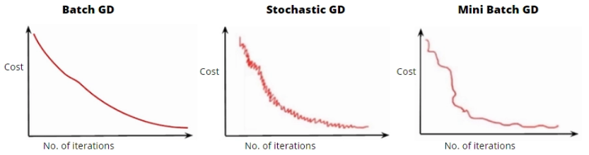
Image Source: https://www.geeksforgeeks.org/ml-mini-batch-gradient-descent-with-python/

• BGD - The average of gradients of all the dataset, the loss function is relatively smooth.
• SGD - The loss function fluctuates from epoch to epoch due to the only using one sample per epoch, making it more volatile.
• MBGD - The balance between speed of convergence and noise associated with gradient update.